CortexFlow: Benchmarking Classical and Neural Sequence Models for Neural Population Dynamics
Gary Wang
Research benchmark. Every number in this manuscript is generated from the
released result files (results/analysis.json); the build fails if any value
cannot be resolved.
Abstract
Modern neural sequence models are routinely applied to neural population recordings, but the protocols they are judged by often let a model see part of the answer: held-out trials interleaved in time with training trials, inference that conditions on the whole trial, smoothing that mixes future bins into the present. We ask a narrower question under a stricter protocol — how much do such models improve on classical dynamical models when the test period is strictly in the future, and when the test animal is one the model has never seen?
We benchmark trivial, classical (per-unit autoregression, ridge vector autoregression, PCA + VAR, a linear-Gaussian state-space model with Kalman filtering) and neural forecasters (RNN, GRU, LSTM, temporal convolutional network, causal transformer) on 936 visual-cortex units from 8 Allen Brain Observatory Neuropixels sessions, 8 mice, at 0.05 s resolution. Each natural movie is presented in two blocks per session, so training on the earlier block and testing on the later one makes the holdout both future and stimulus-matched. Five hypotheses and their decision rules were frozen before the final experiments.
The best one-step forecaster is the simplest model that uses the past: a per-unit autoregression with no population coupling (R² = 0.187), first in 8 of 8 sessions. The best neural model trails the best classical one by ΔR² = −0.033 (−0.053 to −0.013), and the deficit widens as training data shrink, to −0.091 at 10% of the training period. Free rollouts separate the families further: every neural model falls below the mean-rate predictor within 0.35–0.75 s, while no classical model does so within 2.5 s, and the one-step ranking barely predicts the long-horizon one (Spearman 0.26). Transferred to a held-out mouse through an aligned latent space, dynamics retain 85% of within-session skill but the recurrent model's advantage over a linear one disappears. Stimulus covariates do not help one-step prediction and slightly hurt it; their benefit appears only at long horizons, and on grey-screen segments history-only skill remains 75% of its natural-movie value, so most of what is predictable here is not stimulus-locked.
Of the five pre-registered hypotheses, the two favouring neural models were not supported and the three predicting their limits were. The results concern these architectures at this scale, on mouse visual cortex under passive viewing, and are not a claim about neural sequence models in general; the tuning grid's edge was binding, which is reported as a limitation. Code, provenance, frozen decision rules and the full result set are released, and every number in this manuscript and on the accompanying site is generated from those files.
1. Introduction
Recordings of hundreds of simultaneously active neurons invite a dynamical question: given what the population has just done, what will it do next? A model that answers well has captured something about how activity evolves in time. A model that answers well only when it is quietly shown part of the answer has captured nothing at all.
Neural sequence models — recurrent networks, temporal convolutional networks, transformers — are now routinely applied to population recordings. The evaluation protocols they are judged by vary widely. Latent-variable methods such as LFADS infer denoised rates from whole trials, which is smoothing rather than forecasting. Held-out trials are frequently interleaved in time with training trials, so the model is tested on the same stretch of the recording it learned from. Symmetric Gaussian smoothing of spike counts, a common preprocessing step, mixes future bins into the present one. Each of these is defensible for the question it was designed for; none of them tests forecasting.
This benchmark asks a narrower question under a stricter protocol:
How much do modern neural sequence architectures improve neural-population forecasting beyond classical autoregressive and state-space models, when the test period is strictly in the future and when the test animal is new?
We use the Allen Brain Observatory Visual Coding Neuropixels recordings, which offer something unusual: each natural-movie stimulus is presented in two blocks separated by tens of minutes within the same session. Training on the earlier block and testing on the later one yields a holdout that is both in the future and stimulus-matched. We compare 8 sessions from 8 mice across trivial, classical and neural forecasters, on one-step and multi-step forecasts under teacher forcing and free rollout, and test transfer to held-out animals in a stimulus-aligned latent space.
Five hypotheses were fixed before the final experiments (Section 8.1), together with the mechanical rules that decide them. Several of the results are negative for the more complex models. They are reported as they came out.
2. Related work
Latent dynamical models of populations. Low-dimensional linear dynamics have been a productive description of population activity, from rotational structure in motor cortex (Churchland et al., 2012) to the dynamical-systems view reviewed by Vyas et al. (2020). Gaussian-process factor analysis (Yu et al., 2009) and Poisson linear dynamical systems (Macke et al., 2011) extract smooth latent trajectories; LFADS (Pandarinath et al., 2018) and Neural Data Transformers (Ye & Pandarinath, 2021) infer single-trial rates with deep networks. These methods are typically evaluated on inference, where the model may condition on the entire trial.
Benchmarks. The Neural Latents Benchmark (Pei et al., 2021) standardised evaluation across four datasets, with co-smoothing of held-out neurons, a short forward-prediction window and behavioural decoding. Lu et al. (2025) benchmark probabilistic deep and classical forecasters on widefield imaging of spontaneous mouse cortical activity. In general time-series forecasting, Zeng et al. (2023) showed that single-layer linear models frequently match or beat transformer forecasters under strict evaluation.
Stability across time and animals. Latent-space alignment has been used to stabilise decoders across days (Gallego et al., 2020; Degenhart et al., 2020). In mouse visual cortex, responses to repeated natural movies drift over time (Deitch et al., 2021; Marks & Goard, 2021), and a large share of activity covaries with spontaneous behaviour such as running (Stringer et al., 2019). Both facts matter here: a late test block may differ from the early training block for reasons unrelated to any model.
This work. CortexFlow focuses on causal forecasting of single-unit spiking,
under a stimulus-matched future holdout, with free rollouts reported separately
from teacher forcing and with few-shot transfer to held-out animals. It makes no
decoding claim. Bibliographic entries not verified online during the build are
marked in research/literature_matrix.csv.
3. Dataset
We use the Allen Brain Observatory Visual Coding Neuropixels dataset (Siegle et al., 2021), distributed as DANDI:000021 under spdx:CC-BY-4.0 and accessed on 2026-09-11. Files are read by HTTP range requests; only the units table, the spike times of selected units, stimulus interval tables and running speed are transferred, and no raw data are redistributed.
We take the first 8 sessions in subject order, one per mouse, so that every cross-session comparison is also a cross-animal comparison. Of 19,701 sorted units across these sessions, 4,983 pass the quality criteria (Section 4), and after restricting to visual cortex and capping at 120 per session we analyse 936 units (96–120 per session) from areas VISal, VISam, VISl, VISmma, VISp, VISpm, VISrl.
Segments. The analysis uses the two natural-movie stimuli
(natural_movie_one, a 30 s clip; natural_movie_three, a 120 s clip) and
spontaneous grey-screen periods of at least 60 s. Each movie is shown in two
blocks per session. Per session this gives on average
1551 s of recording before the epoch boundary and
1201 s after it (Figure Figure 1).
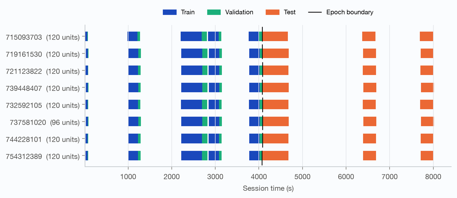
Figure 1. Analysis segments per session. Natural-movie and long spontaneous segments recorded before the epoch boundary supply training (first 80%) and validation (last 20%); segments after it are test. Each movie appears in both epochs, so the future-time holdout is stimulus-matched.
Flagged intervals. The NWB files mark experimenter-flagged invalid intervals. These are tagged either per probe or per session. Units on a probe flagged during any analysis segment are excluded (3 sessions affected); session-wide flags are masked in time, so no window of any split reads a flagged bin.
A complete, programmatically generated account of sessions, subjects,
per-criterion unit exclusions and segment timings is in
research/dataset_provenance.md.
4. Preprocessing
Binning. Spike times are counted once at 10 ms and coarsened by summation to 0.02, 0.05, 0.1 s; the primary resolution of 0.05 s was fixed before any model was compared. Coarsening a single fine assignment, rather than re-binning, means the resolution sweep differs only in resolution.
Unit quality control. Units must be labelled good and satisfy ISI
violations ≤ 0.5, amplitude
cutoff ≤ 0.1, presence
ratio ≥ 0.9, session firing
rate ≥ 0.5 Hz and SNR ≥
1.0, and must sit in visual cortex. At
most 120 units per session are kept, ranked by presence ratio and firing rate —
an ordering independent of any model. Every exclusion is counted.
Normalisation. Each unit is z-scored with statistics from training bins only. The primary transform is the identity, which is exactly invertible. A square-root transform is available as a sensitivity arm; because the naive inverse of a square root under-predicts counts by Var(√y), the second-order retransformation term is added back, estimated from training residuals. In a preliminary run without that correction, the trivial mean-rate predictor scored R² = −0.11 where it must score 0, and every model was penalised in proportion to its residual variance.
No symmetric smoothing. Convolving counts with a symmetric kernel mixes future bins into the present, which is leakage under a forecasting protocol. Only one-sided kernels exist in the code, and none is used by default.
Covariates. Per bin: stimulus-condition indicators; a Fourier code (eight harmonics) of the position within the movie clip, derived from per-frame presentation times; and running speed. The clip-phase code identifies which frame is on screen. It does not describe image content.
5. Forecasting tasks
Split. One epoch boundary per session is set at the start of the earliest late movie block. Segments ending before it supply training (first 80% of each segment) and validation (last 20%, after an embargo of one context length); segments starting after it are test, in full; segments straddling it are discarded. A validator rejects any plan in which a split is empty, a validation bin precedes a training bin, a segment mixes test with training bins, or test time overlaps training time. A window is admissible only if every bin it reads or predicts carries its own split's code, so windows can neither straddle a split boundary nor cross a segment join.
One-step forecast (primary). From 40 bins (2 s) of population activity, predict the spike counts of every unit in the next bin.
Multi-step forecast. Horizons up to 50 bins (2.5 s) under two protocols that share one code path:
- teacher forcing — the model receives the true activity preceding each predicted bin, so an h-step result is h independent one-step forecasts;
- free rollout — the model receives one context window and thereafter consumes its own predictions.
A test asserts that the two coincide at h = 1 and that free rollout is strictly harder than teacher forcing on a noisy synthetic system.
Cross-session forecast. Leave one session out; forecast its test block using dynamics learned on the other sessions (Section 10).
6. Models
All models implement one primitive — predict the next bin from a window of history — and are wrapped by the same rollout and evaluation code.
Trivial. Mean rate (the training-set mean of each unit; the zero of every skill score); persistence (repeat the last bin); smoothed persistence (an exponentially weighted average of the context, one decay parameter tuned on validation).
Classical. AR (per unit): ridge autoregression of each unit on its own past, so it cannot use population coupling. VAR (ridge): multivariate autoregression across all units. PCA + VAR: project to a low-dimensional principal subspace fitted on training bins, autoregress there, reconstruct. LDS (Kalman): a linear-Gaussian state-space model initialised from PCA, fitted by expectation–maximisation on training windows, and forecast with the Kalman filter — never the smoother, which conditions on the future. Classical models tune lag, ridge penalty and latent dimension per session on validation.
Neural. A vanilla RNN, GRU, LSTM, a TCN with dilated causal
convolutions, and a compact causal transformer with a strictly upper-
triangular attention mask. All share one training loop (AdamW, cosine schedule,
gradient clipping, early stopping on validation MSE), one input projection and
a linear readout. Four capacity/regularisation configurations per architecture
were scored on the validation periods of two sessions; the chosen configuration
is recorded in results/tuning.json. Tests probe the TCN and transformer
encoders directly to confirm that changing future inputs cannot change a
prefix's representation.
Stimulus-locked references. A PSTH predictor ignores history and outputs the training-period mean response at the current clip frame. PSTH + residual VAR adds a ridge VAR fitted to the residuals from the PSTH. These appear only in the stimulus-conditioned arm.
Budget accounting. Every run records parameter count, epochs, wall-clock fit time and device in its manifest (Figure Figure 2).
7. Evaluation
Metric space. All metrics are computed on spike counts after mapping predictions back from normalised space. The headline skill score is
R²_train = 1 − Σ(y − ŷ)² / Σ(y − ȳ_train)²,
referenced to the training-period mean rate of each unit. Referencing the test mean would credit a model with the test period's average, which it does not have. Correlation, explained variance, MSE, MAE, Poisson deviance and Poisson negative log-likelihood are also recorded.
Aggregation. Every metric is computed per unit and summarised both as an unweighted mean over units and as a firing-rate-weighted mean, alongside medians and quartiles, so that a few high-rate units cannot carry a result unseen. Neural models are averaged over seeds before aggregation.
Uncertainty. Adjacent bins are strongly dependent, so confidence intervals come from a bootstrap that resamples whole sessions (for session-level summaries) or resamples units within resampled sessions (for unit-level comparisons) — never individual bins. Comparisons are paired. We report mean differences, 95% percentile intervals and paired effect sizes (d_z). Where a Wilcoxon signed-rank p-value is shown it treats pairs as independent and is descriptive; Holm correction is applied across the neural-vs-classical family.
Selection without test access. When a family's "best" model is needed, it is chosen per session by validation score, never by test score.
Structure diagnostics. On contiguous one-step test predictions we compare Welch power spectra, autocorrelation functions and population covariance with the recorded counts. Because conditionally independent Poisson noise inflates only the diagonal of a covariance matrix, the off-diagonal covariance of the counts is an unbiased target for the off-diagonal covariance of a rate forecast; we report the slope of predicted on recorded off-diagonal entries.
Failure taxonomy. Thresholds for high-rate under-prediction, missed population transients, clip-onset failure, rare-pattern failure, rollout divergence, correlation collapse, severe over-smoothing and session-shift drop were frozen before the final runs.
8. Results
8.1 Hypotheses at a glance
Each hypothesis was fixed, together with the mechanical rule that decides it, before the benchmark produced a result. The table is generated from the result files by those rules; the rows fill in as experiment arms complete.
Table 1. Pre-registered hypotheses, their frozen decision rules and the verdicts computed from the result files.
| Hypothesis | Decision rule (frozen) | Verdict | |
|---|---|---|---|
| H1 | Neural sequence models beat linear AR on one-step forecasting. | best-neural minus best-classical (both chosen on validation), session-level bootstrap CI > 0 | not supported |
| H2 | Classical models are competitive or better with little data. | neural-minus-classical gap < 0 at the smallest training fraction AND gap increases with data (Spearman > 0) | supported |
| H3 | Neural-vs-linear gap narrows or reverses across sessions. | (GRU-VAR gap, cross-aligned) minus (GRU-VAR gap, within), target-session bootstrap CI < 0 | supported |
| H4 | Long rollouts expose instability invisible at one step. | Spearman(rank at h=1, rank at h=max, free rollout) < 0.7 OR any model diverges (lowest free-rollout R² over horizons < −1). The divergence clause replaced an amplitude-based collapse/explosion measure that was mis-specified (decision log D-018); the rank-correlation clause is unchanged. | supported |
| H5 | Stimulus covariates improve prediction, mostly at long horizons, and mostly where there is a stimulus. | mean stimulus gain > 0 on movie segments AND gain at h=max > gain at h=1 for every tested model AND spontaneous gain < movie gain | not supported |
8.2 One-step forecasting
The best one-step forecaster of mouse visual-cortex population activity, on a block recorded tens of minutes after training, is the simplest model entered that uses the past at all: a per-unit autoregression, in which each neuron is predicted only from its own recent history. It reached R² = 0.187 (95% session-bootstrap interval 0.172 to 0.201) and was the best history-only model in 8 of 8 sessions. Second was smoothed persistence, an exponentially weighted average of the context with a single tuned parameter (R² = 0.160). Table 2 and Figure 3 give every model.
Table 2. One-step skill on the held-out future block, history-only models: mean over sessions with 95% session-bootstrap interval; neural models averaged over seeds.
| Model | Family | R² (mean, 95% CI) | Median unit R² | Corr. | Params | Fit (s) |
|---|---|---|---|---|---|---|
| AR (per unit) | classical | 0.187 [0.172, 0.201] | 0.169 | 0.372 | 3,960 | 29 |
| Smoothed persistence | trivial | 0.160 [0.144, 0.175] | 0.142 | 0.343 | 1 | 0 |
| VAR (ridge) | classical | 0.144 [0.123, 0.166] | 0.135 | 0.341 | 57,720 | 8 |
| GRU | neural | 0.142 [0.124, 0.163] | 0.131 | 0.340 | 715,896 | 62 |
| Transformer | neural | 0.138 [0.120, 0.158] | 0.122 | 0.333 | 1,247,608 | 66 |
| TCN | neural | 0.130 [0.115, 0.146] | 0.117 | 0.323 | 1,534,328 | 55 |
| LSTM | neural | 0.123 [0.106, 0.141] | 0.109 | 0.316 | 944,248 | 35 |
| RNN | neural | 0.123 [0.108, 0.138] | 0.110 | 0.314 | 259,192 | 67 |
| PCA + VAR | classical | 0.103 [0.088, 0.119] | 0.099 | 0.300 | 12,184 | 1 |
| LDS (Kalman) | classical | 0.086 [0.079, 0.094] | 0.068 | 0.252 | 16,952 | 14 |
| Mean rate | trivial | 0.000 [0.000, 0.000] | 0.000 | 0.000 | 120 | 0 |
| Persistence | trivial | −0.472 [−0.505, −0.440] | −0.492 | 0.225 | 0 | 0 |
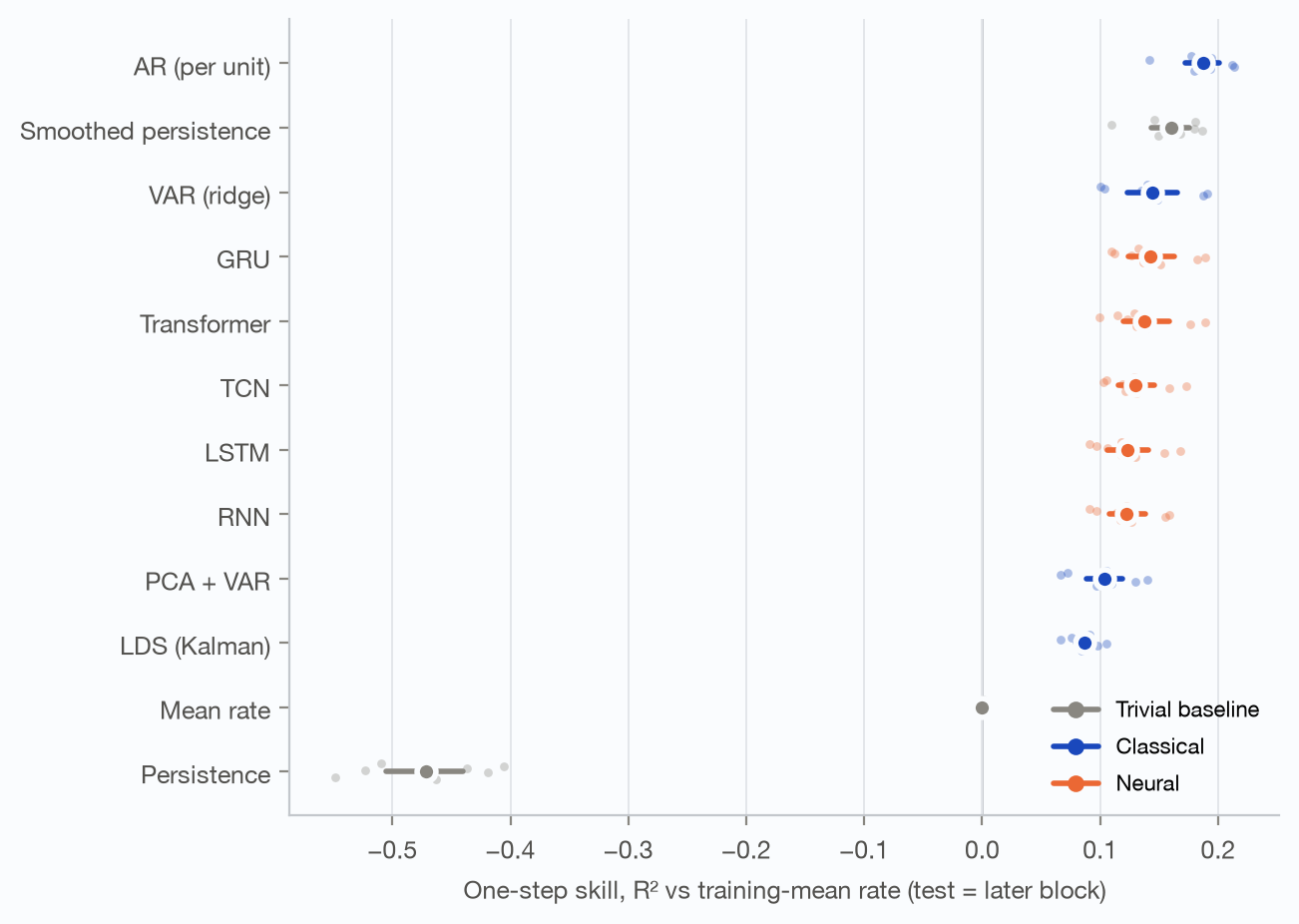
Figure 3. One-step forecast skill on held-out future blocks, history-only models. Faint dots: individual sessions (seed-averaged); large dot and bar: mean over sessions with 95% session-bootstrap CI. Zero is the training-mean-rate predictor.
Neural sequence models did not beat classical ones. Choosing each family's entrant per session by validation score — a GRU in 8 of 8 sessions for the neural family; per-unit AR in 5 and ridge VAR in 3 for the classical family — the best neural model trailed the best classical model by ΔR² = −0.033 (95% interval −0.053 to −0.013; paired d_z = −1.02), and was ahead in only 1 session. H1 is therefore not supported; the interval excludes zero in the opposite direction.
Against per-unit AR specifically, every neural architecture lost: the paired deficits ranged from −0.045 to −0.065, all 5 of 5 intervals lay below zero, and at best a neural model won 0 of the 8 head-to-head sessions against it. The best neural models were close to ridge VAR rather than to the univariate model: GRU minus VAR was −0.0016 (−0.0060 to +0.0034), and the causal transformer minus VAR was −0.0063. The same pattern holds unit by unit (see the site's models page; Table 3 gives the session-level comparisons), where intervals resample units within resampled sessions.
Table 3. Session-level paired differences in one-step R² (A − B). Intervals resample sessions; d_z is the mean difference over the SD of differences.
| Comparison (A vs B) | Mean ΔR² | 95% CI | d_z | A better in | n |
|---|---|---|---|---|---|
| Best neural vs best classical (validation-selected) | −0.0328 | [−0.0529, −0.0127] | −1.02 | 12% | 8 |
| RNN vs AR (per unit) | −0.0646 | [−0.0774, −0.0541] | −3.48 | 0% | 8 |
| RNN vs VAR (ridge) | −0.0214 | [−0.0275, −0.0153] | −2.20 | 0% | 8 |
| RNN vs Smoothed persistence | −0.0378 | [−0.0549, −0.0239] | −1.52 | 0% | 8 |
| GRU vs AR (per unit) | −0.0448 | [−0.0591, −0.0325] | −2.15 | 0% | 8 |
| GRU vs VAR (ridge) | −0.0016 | [−0.0060, +0.0034] | −0.21 | 38% | 8 |
| GRU vs Smoothed persistence | −0.0180 | [−0.0361, −0.0022] | −0.67 | 38% | 8 |
| LSTM vs AR (per unit) | −0.0644 | [−0.0784, −0.0524] | −3.18 | 0% | 8 |
| LSTM vs VAR (ridge) | −0.0212 | [−0.0268, −0.0154] | −2.32 | 0% | 8 |
| LSTM vs Smoothed persistence | −0.0376 | [−0.0560, −0.0220] | −1.42 | 0% | 8 |
| TCN vs AR (per unit) | −0.0574 | [−0.0692, −0.0468] | −3.29 | 0% | 8 |
| TCN vs VAR (ridge) | −0.0141 | [−0.0210, −0.0066] | −1.23 | 12% | 8 |
| TCN vs Smoothed persistence | −0.0306 | [−0.0465, −0.0166] | −1.30 | 0% | 8 |
| Transformer vs AR (per unit) | −0.0495 | [−0.0614, −0.0383] | −2.78 | 0% | 8 |
| Transformer vs VAR (ridge) | −0.0063 | [−0.0114, +0.0000] | −0.69 | 12% | 8 |
| Transformer vs Smoothed persistence | −0.0227 | [−0.0387, −0.0087] | −0.96 | 12% | 8 |
These gaps are not an artefact of seed choice or of a starved parameter budget. Across three seeds the session-level standard deviation of a neural model's R² was at most 0.0030, an order of magnitude below the gaps. The neural models carried 65–387 times as many parameters as the per-unit AR (3,960; Figure 2). As noted in Section 6, however, every architecture chose the largest configuration on its tuning grid, so the networks may sit below their ceiling; Section 8.5 measures how much width would have helped.
A note on inference. With eight sessions the smallest two-sided Wilcoxon signed-rank p-value attainable is 0.0078, so after Holm correction across the fifteen neural-versus-classical comparisons no adjusted p-value can fall below 0.117 — the floor was reached. The session-bootstrap intervals, declared in advance as the primary inference, carry the conclusions above; the rank-test p-values are reported as descriptive.
Skill is uneven across neurons. The median unit's R² sat below the mean for every model (Figure 4), and skill rose with firing rate for all of them alike (Spearman ρ between 0.27 and 0.34; Figure 5): at 50 ms, a unit firing a few spikes per second is close to unpredictable by any model here. Rate-weighted means are higher than unweighted ones for every model and are reported alongside them.
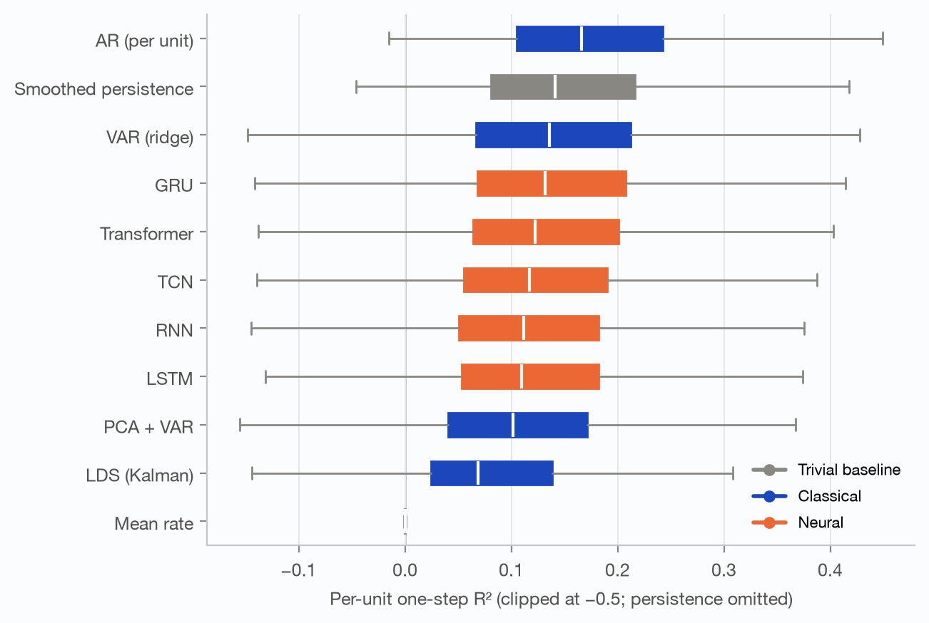
Figure 4. Distribution of one-step skill across all units in all sessions. Boxes: interquartile range; white line: median; whiskers: 1.5 IQR. Population means hide a long lower tail.
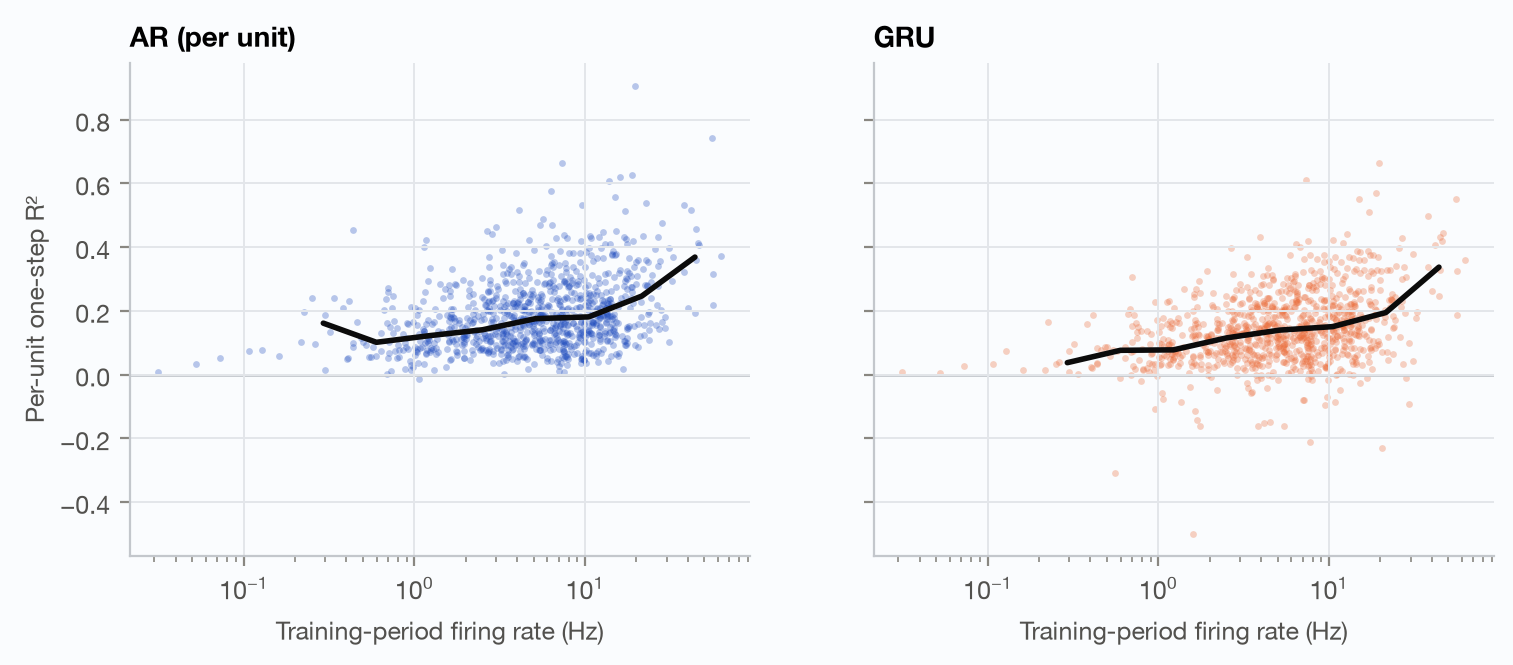
Figure 5. Per-unit skill against firing rate (log scale). Dots: units; black line: binned median. Low-rate units are close to unpredictable at 50 ms.
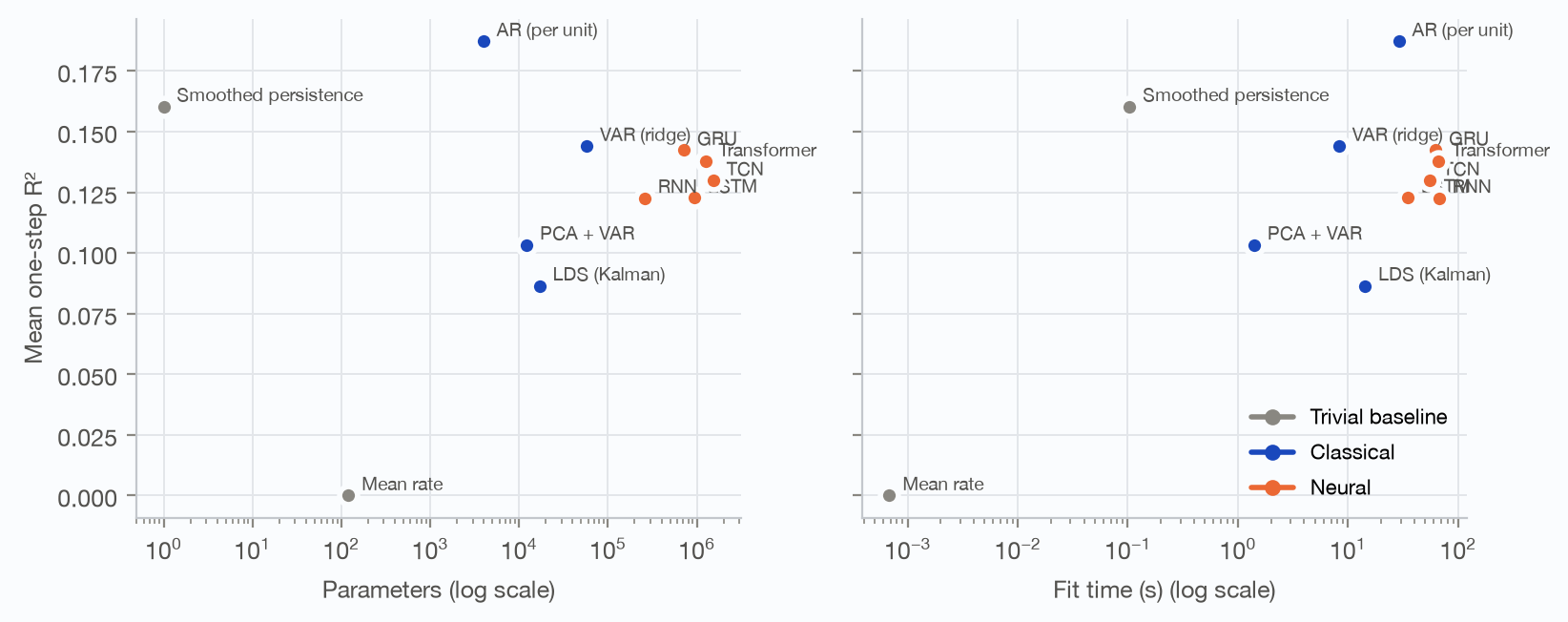
Figure 2. Cost against skill. Parameter count and wall-clock fit time (Apple-silicon MPS for neural models, CPU for classical) against mean one-step skill.
8.3 What a good one-step score hides
All forecasts are smoother than the counts they predict — by construction, since the Poisson component of spiking cannot be forecast. At 4–10 Hz the forecasts carried between 0.00 and 0.07 of the recorded power (Figure 6), and their covariance spanned 4–11 effective dimensions against 32 for the counts.
The informative comparison is the off-diagonal structure, which independent Poisson noise leaves untouched. Here the ranking of Section 8.2 is partly reversed and partly confirmed. The per-unit AR, which has no cross-unit coupling at all, reproduced the pattern of pairwise correlations more faithfully than any neural model or ridge VAR (similarity 0.90, against 0.68–0.73 for the neural models and 0.77 for VAR; the trivial persistence forecast, which copies counts, reproduces them exactly and is excluded from this comparison): shared fluctuations are visible in each neuron's own recent past, so a model of that past inherits them. But it reproduced their magnitude least well (off-diagonal covariance slope 0.42, against 0.57 for ridge VAR), and it missed population-wide transients in 100% of sessions, where ridge VAR missed them in 12% (Section 12). The best one-step model is not the best model of joint population events.
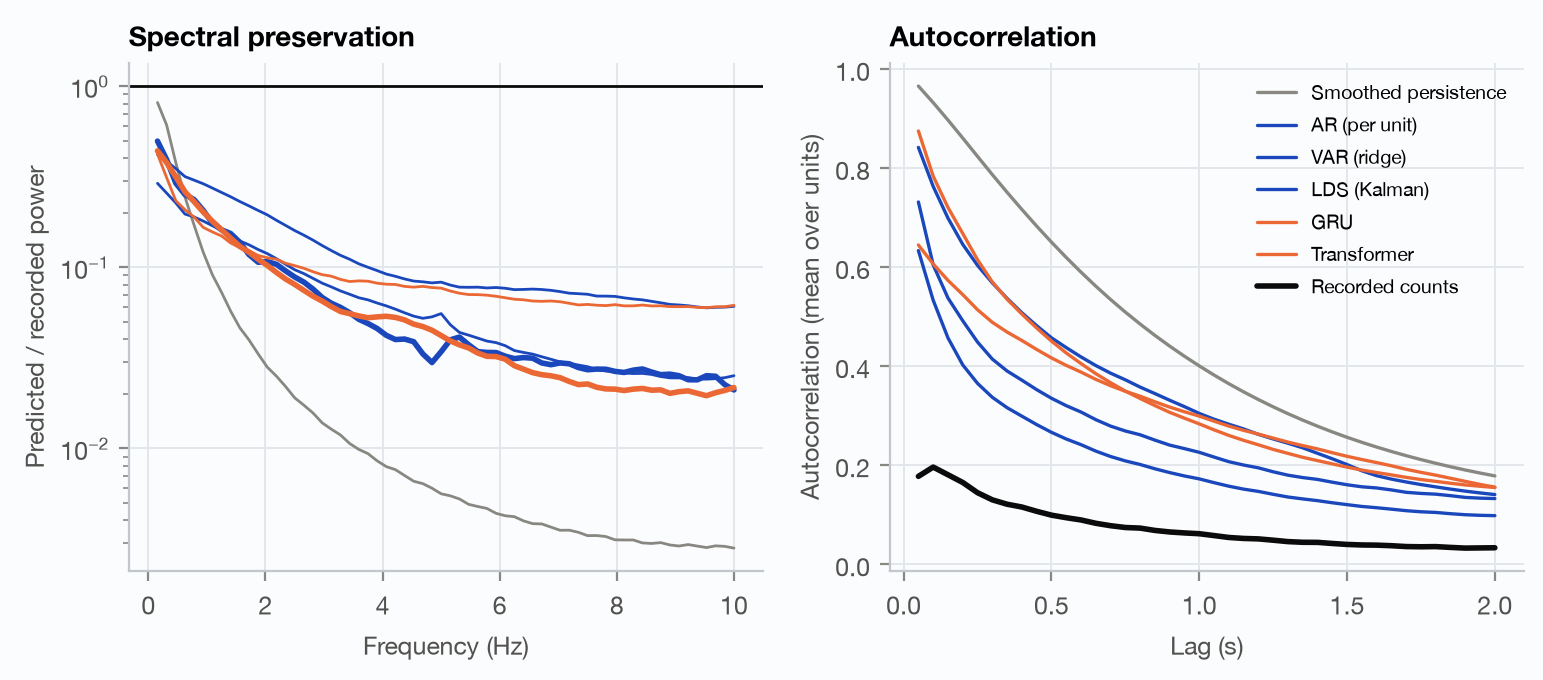
Figure 6. Temporal structure of one-step predictions vs recorded spike counts on test blocks. Any rate forecast is expected to carry less high-frequency power than counts (the Poisson component is unpredictable); the question is how much slow structure survives.
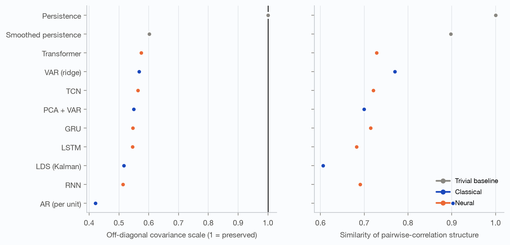
Figure 7. Does the forecast reproduce joint population structure? Left: slope of predicted on recorded off-diagonal covariance (independent Poisson noise does not bias the off-diagonal, so 1 is the target). Right: correlation between predicted and recorded pairwise-correlation matrices.
Table 4. Structure of one-step forecasts against recorded counts on test blocks. Values are means over sessions.
| Model | Power ratio 4–10 Hz | Log-PSD corr. | Off-diag. cov. scale | Corr.-structure similarity | Participation ratio (pred / true) |
|---|---|---|---|---|---|
| AR (per unit) | 0.031 | 0.902 | 0.421 | 0.903 | 10.5 / 32.4 |
| GRU | 0.029 | 0.871 | 0.546 | 0.714 | 6.4 / 32.4 |
| LDS (Kalman) | 0.035 | 0.876 | 0.516 | 0.606 | 4.0 / 32.4 |
| LSTM | 0.024 | 0.861 | 0.546 | 0.682 | 5.9 / 32.4 |
| PCA + VAR | 0.032 | 0.918 | 0.550 | 0.700 | 4.9 / 32.4 |
| Persistence | 1.000 | 1.000 | 1.000 | 1.000 | 32.4 / 32.4 |
| RNN | 0.043 | 0.912 | 0.514 | 0.691 | 5.9 / 32.4 |
| Smoothed persistence | 0.004 | 0.910 | 0.602 | 0.898 | 9.7 / 32.4 |
| TCN | 0.072 | 0.956 | 0.564 | 0.721 | 6.4 / 32.4 |
| Transformer | 0.067 | 0.966 | 0.575 | 0.728 | 6.6 / 32.4 |
| VAR (ridge) | 0.073 | 0.906 | 0.567 | 0.770 | 7.9 / 32.4 |
8.4 What the stimulus explains
The movies repeat, so a model could score well by learning what each neuron does at each frame rather than by capturing anything about how activity evolves. Three comparisons separate those (Figure 8, Table 5).
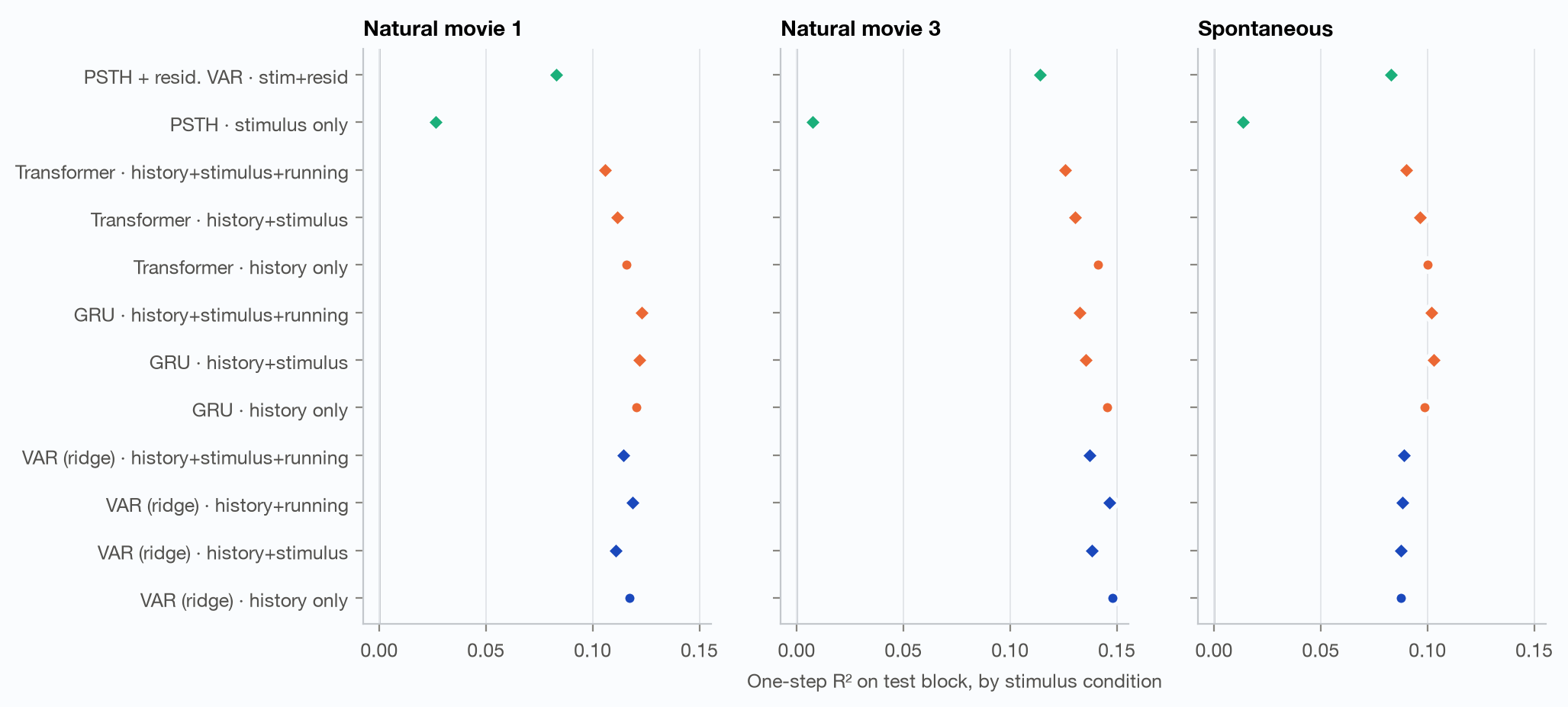
Figure 8. Covariate ablation. Circles: neural history only; diamonds: history plus covariates. Aqua: stimulus-locked references (PSTH ignores history entirely). Comparing the movie panels with the spontaneous panel separates stimulus-locked predictability from predictability that persists without a stimulus.
The stimulus-locked response alone is small at 50 ms. The PSTH predictor, which ignores neural history entirely and outputs the training-period mean response at the current frame, reached R² = 0.018 — against 0.187 for the best history-only model. Whatever the forecasters are exploiting at one step, it is mostly not the repeated stimulus.
Telling a model the stimulus does not help it, and slightly hurts. Adding the clip-phase code to a model that already has neural history changed one-step skill by between −0.0105 and +0.0012 on movie segments; 4 of 6 comparisons were reliably negative and 0 were reliably positive. On spontaneous segments, where the code carries no information beyond "grey screen", the changes were null (−0.0035 to +0.0044, 0 of three intervals excluding zero). The straightforward reading is that two seconds of population history already tells the model where in the clip it is, so the explicit code adds parameters rather than information.
At long horizons the sign flips. In free rollout the stimulus code was worth +0.009 to +0.025 at 2.5 s, and the gain grew with horizon for 3 of 3 models tested. The PSTH makes the mechanism plain: because it never consumes its own output, it does not degrade at all — 0.018 at one step and 0.023 at 2.5 s — so by the longest horizon it is ahead of every neural model (all of which are below zero there, Section 9) and close to the best classical one. Stimulus knowledge is not what makes a good one-step forecast; it is what is left when the history a model was given has been used up.
Most of the predictability is not stimulus-locked. On spontaneous grey-screen segments, with no clip to lock to, the best history-only model still reached R² = 0.155, against 0.206 on natural movie one — that is 75% of the movie figure. Prediction here rests mainly on the population's own recent past, not on the experiment's schedule.
H5 is therefore not supported as stated. Its clause about horizon held — the gain does grow with horizon, for every model tested — but its first clause, that the stimulus code improves prediction on movie segments, did not: the mean movie gain was −0.0066. The corollary the hypothesis was designed to guard against does not arise, because the stimulus-conditioned models never bought an advantage at one step that could have been mistaken for autonomous dynamics.
Table 5. Gain in one-step R² from adding the stimulus code to the same model, paired by session.
| Model | Condition | Stimulus gain ΔR² | 95% CI | n sessions |
|---|---|---|---|---|
| GRU | nm1 | +0.0012 | [−0.0099, +0.0176] | 8 |
| GRU | nm3 | −0.0100 | [−0.0146, −0.0053] | 8 |
| GRU | spont | +0.0044 | [−0.0006, +0.0117] | 8 |
| Transformer | nm1 | −0.0042 | [−0.0105, +0.0002] | 8 |
| Transformer | nm3 | −0.0105 | [−0.0174, −0.0056] | 8 |
| Transformer | spont | −0.0035 | [−0.0075, +0.0012] | 8 |
| VAR (ridge) | nm1 | −0.0064 | [−0.0126, −0.0009] | 8 |
| VAR (ridge) | nm3 | −0.0098 | [−0.0140, −0.0067] | 8 |
| VAR (ridge) | spont | +0.0000 | [−0.0009, +0.0010] | 8 |
8.5 Does the ranking survive the choices we made?
Section 8.2 measured one configuration: the full training period, each architecture's tuned width, 50 ms bins, and one unit-selection rule. Each of those is a choice that could be carrying the result. This section varies them in turn, on subsets of sessions, and asks only whether the ordering moves.
More data narrows the gap, and it was still narrowing at the end of the recording. Refitting each model on the most recent contiguous 10%, 30% and 100% of the training period, on 4 sessions, the best-neural minus best-classical gap ran from −0.091 (−0.097 to −0.086) at the smallest fraction to −0.037 at the full period, closing monotonically (Spearman 1.00; Figure 9). What moves is how much each model loses when data are removed, and it does not fall along family lines: at 10% of the training period the per-unit AR still retained 92% of its full-data skill, while the GRU (53%) and ridge VAR (43%) degraded comparably and the transformer kept only 15%. What separates them is how many parameters each must estimate from the shortened record, not whether it is classical or neural. This is H2's clause and it is supported. What it does not license is extrapolation: the trend is consistent with the gap closing given more data than a session contains, and these recordings cannot say where, or whether, it would reach zero.
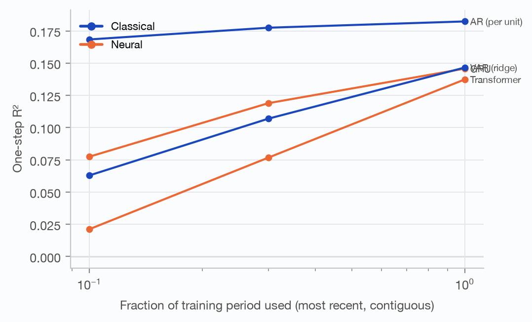
Figure 9. Data scaling. Each model is refit on the most recent contiguous fraction of the training period; validation and test are unchanged.
Width does not close the gap, and the deficit is not a starved-budget artefact. Holding everything else at the tuned configuration and varying only the hidden width across 32, 128 and 512 units on 3 sessions, the GRU improved throughout — 0.107 at the narrowest to 0.161 at the widest — while the transformer peaked at 128 units (0.148) and fell back to 0.144 at 512 (Figure 10). The comparison that matters is against the same sessions' classical baseline, not the headline mean: the per-unit AR scored 0.196 on these sessions, so the best cell anywhere in the sweep — 0.161, the 512-unit GRU at 2,611,320 parameters — still trailed it by −0.035. Two details qualify this. The GRU's best width was the largest tested, so the sweep bounds what width bought here rather than locating a ceiling; and the widest networks stopped early, at a mean best epoch of 4 against 37 at the narrowest width, so the extra capacity was not also being trained for longer. The validation-minus-test drop stayed between 0.022 and 0.029 across every cell with no systematic widening, which is evidence that width was not buying near-future skill that then failed to carry to the later block.
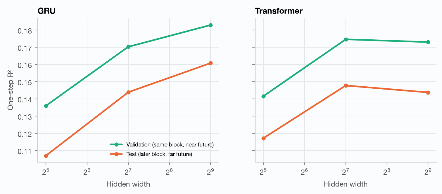
Figure 10. Capacity: does a wider network help in the near future (validation, same stimulus block) more than in the far future (test, a block recorded ~30-60 min later)?
Temporal resolution changes every score and almost nothing about the order. Sweeping 20, 50 and 100 ms bins with context and horizon held fixed in seconds, one-step R² rose with bin width for every model — from 0.104 to 0.282 for the per-unit AR — because coarser bins average away the Poisson component that no model can forecast (Figure 11). Those numbers are therefore not comparable across resolutions, and the interesting quantity is the ranking. The per-unit AR was first at 3 of 3 resolutions, and the rank correlation against the 50 ms ordering was 1.00 at 100 ms and 0.70 at 20 ms, where the only reshuffle is ridge VAR passing the GRU. The classical-minus-GRU margin in fact widened with coarser bins, from +0.027 at 20 ms to +0.064 at 100 ms. The headline comparison is not an artefact of the 50 ms choice.
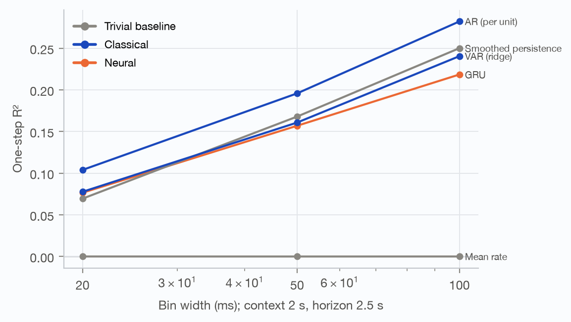
Figure 11. Temporal resolution. One-step skill rises with bin width for every model because coarser bins average away Poisson noise; the question is whether the ranking changes.
Unit selection moves every score and none of the ordering. Rerunning the comparison under 3 alternative selection rules — relaxed quality criteria, strict criteria, and a cap of 60 units — the per-unit AR was first in 4 of 4 settings, the default included. Absolute skill tracked how predictable the retained population was rather than how large it was: capping at the top 60 units by presence ratio and firing rate gave the highest score of the four (0.227), strict criteria (79 units on average) 0.201, and relaxing the criteria to admit lower-rate, less well isolated units 0.196. The objection this arm exists to answer — that quality control keeps the easy neurons and flatters the simple model — runs the opposite way from the result: admitting the harder units widened the classical margin, from +0.025 under strict criteria to +0.047 under relaxed ones. Across all 4 settings that margin stayed between +0.025 and +0.047 and never reversed. The arm ran on three sessions and the models it could afford to refit, so it bounds the ranking's sensitivity to unit selection rather than re-deriving the ranking.
9. Long-horizon dynamics
A forecast that is fed its own predictions is a different object from one that is handed the truth at every step. The two coincide at one step and diverge thereafter (Figure 12, Table 6).
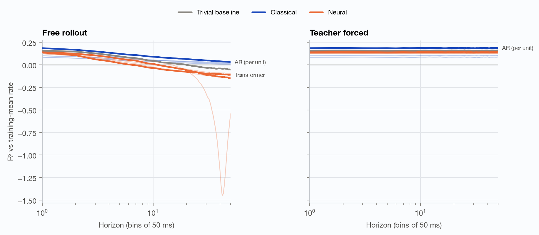
Figure 12. Skill as a function of forecast horizon. Left: free rollout (the model consumes its own predictions). Right: teacher forcing (true history at every step). Thin lines: every model; thick lines: representative models, labelled where labels do not collide. Zero is the mean-rate predictor. Persistence (about −0.5 at one step) is omitted so the remaining curves stay readable; it is in the rollout table.
Classical models decay to the mean; neural models overshoot it. Under free rollout, every neural model fell below the mean-rate predictor — the point at which forecasting is worse than not forecasting — within 0.35 to 0.75 s. None of the 4 classical models did so at any horizon up to 2.5 s: at the longest horizon per-unit AR still scored +0.032 and ridge VAR +0.012. The mechanism is visible in how much each forecast moves. The classical rollouts relax onto the training mean — their temporal variability was 0.08–0.11 of the recorded counts' — which is the minimum-risk behaviour once the future is unpredictable. The neural rollouts keep moving (0.18–0.19, excluding the TCN), but the movement is not aligned with what the population does, so it adds error.
Teacher forcing hides this. At 2.5 s the gap between teacher-forced and free-rollout skill was 0.23–0.68 for the neural models and 0.08–0.16 for the classical ones. A teacher-forced curve at that horizon measures one-step skill fifty times over; reporting it as a long-horizon result would have overstated every neural model by more than it overstated any classical one.
The one-step ranking does not predict the long-horizon ranking. The Spearman correlation between model orderings at one step and at 50 steps was 0.26. One model diverged outright: the TCN's free-rollout skill reached a minimum of −1.45, and it was flagged for divergence in 88% of sessions. H4 is supported on both of its clauses.
Table 6. Free-rollout summary per model. Horizons in 50 ms bins.
| Model | R² at h = 1 | R² at h = 50 (free) | Teacher-forced − free at h = 50 | First horizon ≤ mean-rate |
|---|---|---|---|---|
| AR (per unit) | 0.185 | +0.032 | +0.157 | never |
| Smoothed persistence | 0.157 | −0.053 | +0.214 | 20 |
| GRU | 0.144 | −0.148 | +0.298 | 11 |
| VAR (ridge) | 0.139 | +0.012 | +0.133 | never |
| Transformer | 0.137 | −0.110 | +0.253 | 7 |
| TCN | 0.128 | −0.542 | +0.676 | 15 |
| LSTM | 0.123 | −0.099 | +0.226 | 11 |
| RNN | 0.122 | −0.149 | +0.277 | 8 |
| PCA + VAR | 0.100 | +0.023 | +0.080 | never |
| LDS (Kalman) | 0.084 | +0.005 | +0.082 | never |
| Mean rate | 0.000 | +0.000 | +0.000 | never |
| Persistence | −0.501 | −0.786 | +0.307 | 1 |
10. Generalization across animals
Neurons do not correspond across mice, so transfer is tested in a population latent space: each session gets its own 16-dimensional PCA encoder and decoder fitted on its own training bins, and the spaces are rotated into a common frame by orthogonal Procrustes on movie-locked responses. The target mouse contributes only its training period to that rotation, so this is few-shot transfer, not zero-shot (Figure 13, Table 7).
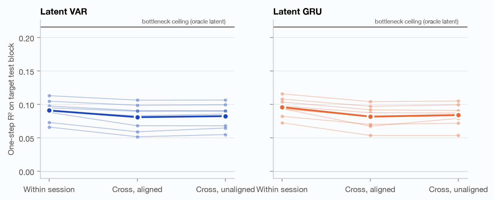
Figure 13. Leave-one-session-out transfer through a K=16 PCA latent space. Thin lines: individual target sessions (each a different mouse); thick line: mean. Alignment uses the target's training period only (few-shot). The horizontal line is the ceiling imposed by the 16-dimensional bottleneck.
Most of the skill survives the move to a new animal. Dynamics fitted on seven mice and applied to the eighth reached R² = 0.081 for the latent VAR and 0.082 for the latent GRU, against 0.091 and 0.096 when the same model was trained on the target's own training period — that is, 89% and 85% of the within-session figure. The drops are small but consistent: the paired loss was +0.0100 (+0.0070 to +0.0137) for the VAR and +0.0140 (+0.0111 to +0.0180) for the GRU, in both cases in every one of the 8 held-out mice.
The neural advantage does not survive it. Inside the bottleneck the GRU was reliably, if slightly, better than the linear model when trained on the target itself (ΔR² = +0.0049, +0.0036 to +0.0064, ahead in 100% of mice). Trained on other animals, that margin fell to +0.0009 (−0.0013 to +0.0040), an interval that includes zero. The difference between the two gaps is −0.0040 (−0.0052 to −0.0022), so H3 is supported: whatever the recurrent model adds within an animal is not what carries across animals.
The alignment did not earn its place. Rotating each session into the shared frame was worse than leaving every session in its own PCA coordinates, by −0.0016 (−0.0030 to −0.0003) for the VAR and −0.0022 for the GRU; both intervals exclude zero. Two things plausibly contribute, and this design cannot separate them. The sessions already share a stimulus, a brain system and a variance-ordered basis, so the unrotated spaces are more comparable than the method assumes. And the rotation itself is fitted to a moving target: the same rotation that matched the training block's movie response at correlation 0.71 matched the test block's at only 0.49. An alignment meant to bridge the gap between animals is subject to the drift between blocks within one animal.
What limits transfer is the dynamics, not the bottleneck. Decoding the true next latent through each session's own decoder — the ceiling the 16 dimensions impose — scores 0.216. The best latent dynamics reach 44% of that within a session and less across animals, so the room being lost is in predicting the latent trajectory, not in the width of the space it lives in.
Table 7. Leave-one-session-out transfer in a 16-dimensional aligned latent space: mean over held-out mice with 95% interval.
| Model | Condition | R² (mean, 95% CI over target sessions) |
|---|---|---|
| latent gru | cross aligned | 0.082 [0.071, 0.093] |
| latent gru | cross unaligned | 0.084 [0.073, 0.094] |
| latent gru | within | 0.096 [0.087, 0.105] |
| latent var | cross aligned | 0.081 [0.068, 0.094] |
| latent var | cross unaligned | 0.083 [0.071, 0.094] |
| latent var | within | 0.091 [0.081, 0.101] |
| oracle | oracle recon | 0.216 [0.187, 0.241] |
11. Latent structure
Low-dimensional descriptions of population activity are usually a modelling choice rather than something the data insist on, and this benchmark is in a position to say how much that choice costs.
Forecast skill did not peak inside the range we swept. Refitting PCA + VAR at each latent dimension, one-step skill rose monotonically from R² = 0.042 at two dimensions to 0.103 at 32, the largest tested (Figure 14). The optimum therefore sits at the sweep's upper edge: these data do not show a low-dimensional bottleneck that is better than using more dimensions, only that skill accumulates slowly as dimensions are added. Even at 32 dimensions the latent model remained below the full-dimensional per-unit AR (0.187).
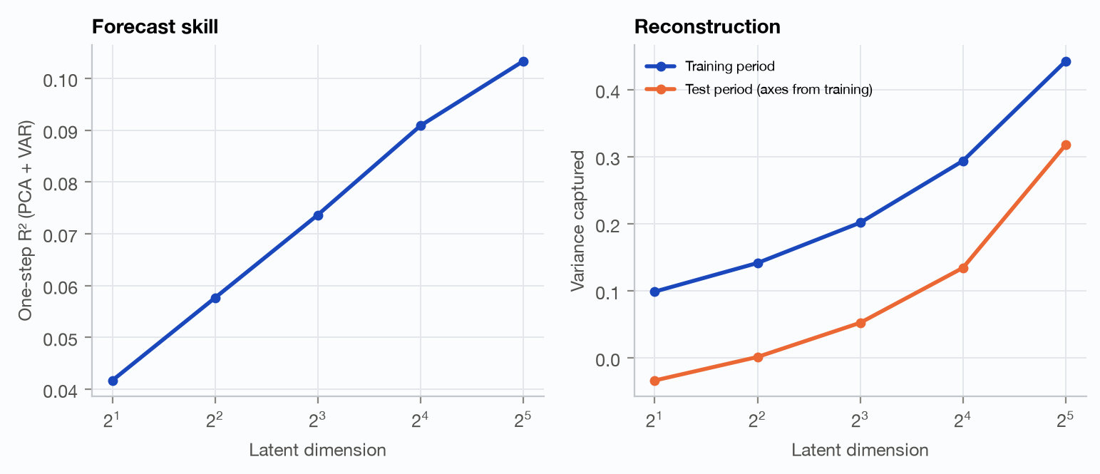
Figure 14. Latent dimensionality. Left: forecast skill of PCA + VAR by dimension. Right: fraction of z-scored population variance captured by training-period axes, in the training and the test period.
The dominant axes move between blocks. Principal axes fitted on the training period captured 0.443 of training variance but only 0.318 of test variance at the same dimension; at two dimensions the test-period reconstruction was −0.034 — worse than predicting the test period's own mean. Comparing subspaces directly, the similarity between the dominant eight-dimensional subspaces of the early and late blocks was 0.561, against 0.680 for two halves of the training period alone — the finite-data floor for this comparison. The gap, +0.119 (+0.028 to +0.223), excludes zero, and the early axes recovered only 50% of the variance that the late period's own axes do. This is descriptive — the late-block PCA is fitted on test bins and feeds nothing that is scored — but it is the same movement that degrades the cross-animal alignment (Section 10) and that any drop from validation to test partly reflects (Section 13).
Latent time constants are short. Fitting a first-order latent model per session and reading its eigenvalues — quantities that do not depend on the basis, so they can be compared across mice without alignment — the slowest mode decayed with a time constant of 0.25 s (0.21 to 0.29), with on average 2.0 oscillatory modes per session. A quarter of a second of memory in the dominant mode is consistent with what the rollouts show: by a second of free running, models that lean on the population's own past have little left to lean on.
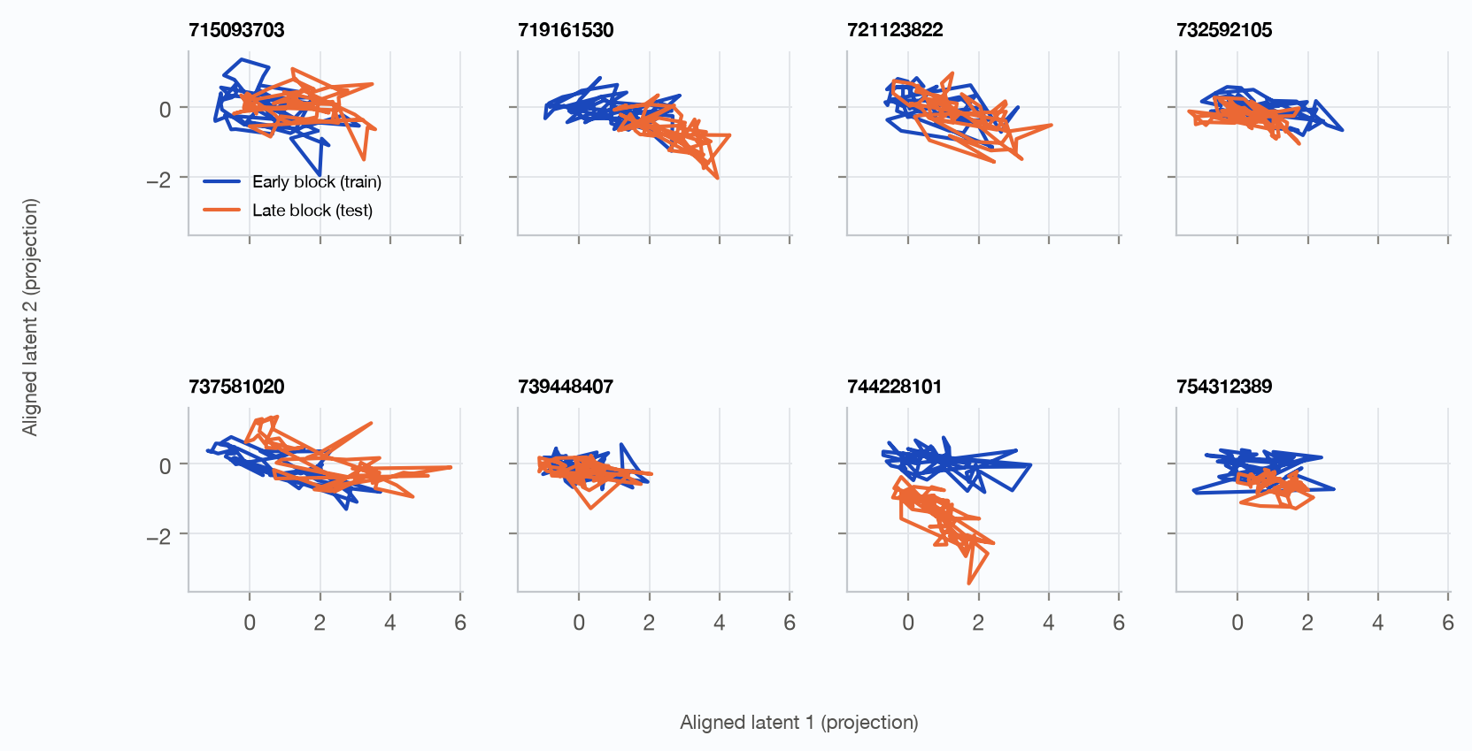
Figure 15. Movie-locked mean population trajectory through natural_movie_one (30 s clip, 0.5 s phase bins) in the first two dimensions of a Procrustes-aligned PCA space. Early block (training period) vs late block (test period). The paths are jagged because each point is a mean over the clip's repeats within one block, not because the population moves that way; what the panels show is the offset between blocks. A projection for visualisation - loops and distances are not evidence of discrete states.
The trajectories above are a projection for looking at, not a result. Distances, loops and apparent clusters in two principal dimensions of a movie-locked average are not evidence of discrete states, and nothing in this section should be read as a claim about what visual cortex computes.
12. Failure analysis
The taxonomy asks where each model fails in a way its average score conceals. Every entry has a statistic and a threshold frozen before the final runs; the flag rate is the share of sessions in which a model trips it (Figure 16).
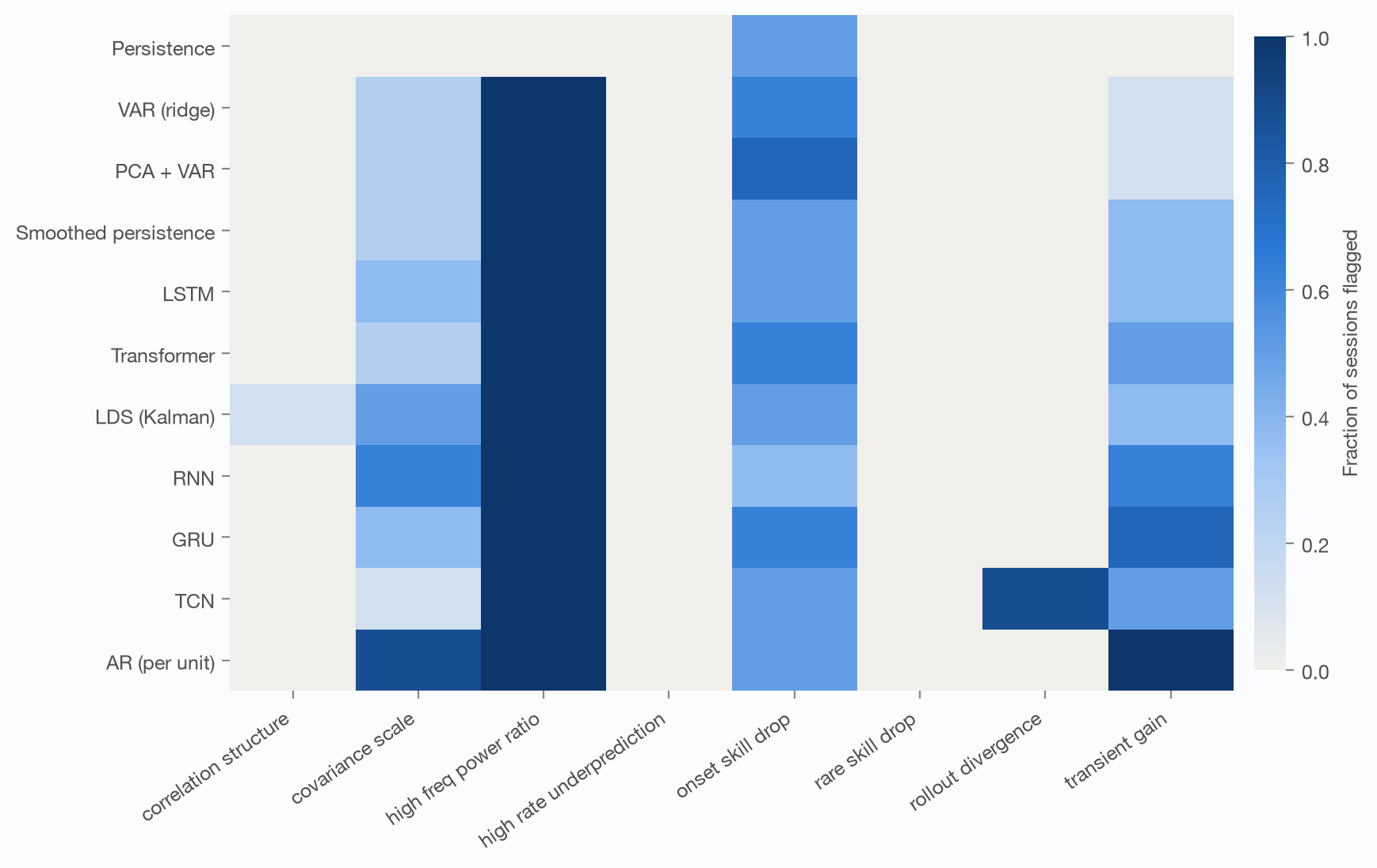
Figure 16. Failure taxonomy: fraction of sessions in which each model trips each pre-registered threshold (cortexflow/failures.py). Thresholds were frozen before the final runs.
Three failure modes appeared, two did not, and one criterion turned out to carry no information.
Population transients. The per-unit AR missed the largest population-wide excursions in 100% of sessions, capturing less than half of their amplitude; ridge VAR and PCA + VAR missed them in 12% and 12%. Coupling across units buys little average skill here but is what lets a model anticipate events that involve the whole population.
Clip onsets. Every forecaster lost disproportionate skill in the half-second after a movie clip restarts in some sessions — between 38% and 75% of them depending on the model. A history-only model cannot know a cut is coming; the stimulus-conditioned arm (Section 8.4) addresses exactly this.
Divergence. Only the TCN tripped the divergence criterion, in 88% of sessions.
Two failure modes did not appear: 0 of 10 forecasters systematically under-predicted their highest-rate units in any session, and 0 of 10 lost disproportionate skill on population patterns that were rare in the training period.
An uninformative criterion. The over-smoothing threshold — predicted power at 4–10 Hz below a quarter of the recorded power — flagged 10 of 10 forecasters, including smoothed persistence. Because the Poisson component of spiking dominates that band and cannot be forecast, the threshold was set too high to discriminate. It is reported as frozen rather than re-tuned after the fact.
13. Limitations
One dataset, one system, one behavioural state. Everything here is mouse visual cortex under passive viewing, 8 sessions from 8 mice. Motor cortex, primates, task-engaged animals and other recording modalities are outside what these data can speak to. The comparison also runs on a single spike-sorting pipeline's output, whose errors are inherited.
Eight animals bound the precision. Session-level intervals rest on n = 8, and the rank-test floor discussed in Section 8.2 means multiplicity-corrected p-values cannot reach conventional thresholds at this sample size. The intervals are shown rather than summarised away, and the per-session sign counts accompany every comparison. Thirty-two sessions are available; the extended tier would use them.
Unit selection favours the predictable. At most 120 quality-controlled cortical units per session are analysed, ranked by presence ratio and firing rate, and skill rises with firing rate for every model (Section 8.2). Low-rate and poorly isolated units — plausibly the hardest — are under-represented. The filtering arm (Section 8.5) tests whether the ranking survives relaxed and strict criteria and a smaller cap, on a subset of sessions.
The networks may sit below their ceiling. Every architecture selected the largest configuration on its tuning grid, so the grid's edge was binding (Section 6). The capacity arm measures whether more width would have closed the gap, but it cannot rule out that a substantially larger model, a different optimiser schedule, or pre-training across sessions would behave differently. The claim defended here is about these architectures at this scale under this protocol, not about neural sequence models in general.
Elapsed time is not the only difference between train and test. The design removes the stimulus confound — the same movie is shown in both blocks — but not arousal, running behaviour or genuine representational drift over the intervening tens of minutes. Section 11 quantifies how far the dominant population axes move; it cannot attribute a model's loss between validation and test uniquely to extrapolation failure.
The stimulus repeats, so "history only" is not "autonomous dynamics". A model given only neural history can still infer where in the clip it is and reproduce the stimulus-locked response. That is why the stimulus-locked references and the spontaneous condition exist (Section 8.4); it remains a caveat on any interpretation of these scores as evidence about internally generated dynamics.
Transfer is few-shot and linearly aligned. The target animal supplies its own PCA space and its training period supplies the rotation. The alignment that was supposed to make spaces comparable did not help (Section 10), which bounds what this experiment establishes: it shows that this alignment, on these sessions, adds nothing, not that latent-space alignment is unnecessary in general. CCA, learned read-in layers and cross-session pre-training are untested here.
Point forecasts, so calibration is not compared. Only the state-space model emits a predictive variance. Uncertainty for every other entrant comes from resampling sessions, not from the model, so the benchmark says nothing about which family is better calibrated.
Entrants that are missing. Sequential auto-encoders of the LFADS family are excluded because their inference is non-causal by construction and would be leakage under this protocol; Gaussian-process dynamics are cubic in series length at these durations; switching linear systems and neural ODEs were not run. Any of them could change the ranking.
Some analysis choices are judgement calls. Failure thresholds were frozen in advance but not derived from first principles, and one of them — the over-smoothing criterion — turned out to flag every forecaster and so carried no information (Section 12). The data-scaling arm shortens the training period but keeps the normaliser fitted on the full one. The rollout-stability measure was found to be mis-specified after the primary arm had run, and because rollout predictions were not stored it could be corrected only by re-deriving divergence from the stored skill curves (decision log D-018).
Finally, what a forecast is. Skill here is statistical structure in binned spike counts. It is not a mechanism, a latent dimension is a coordinate rather than a brain state, and a covariate that improves prediction has not thereby been shown to cause anything.
14. Conclusion
The question was deliberately narrow: when the test period lies strictly later in time, when the stimulus is matched across the split so that elapsed time rather than content separates train from test, and when the test animal may be one the model has never seen, do modern neural sequence models forecast population activity better than classical dynamical models? On 936 visual-cortex units from 8 mice, they do not.
The best one-step forecaster is the simplest model that uses the past: a per-unit autoregression with no cross-unit coupling at all, at R² = 0.187, first in 8 of 8 sessions, with the best neural model behind it by −0.033 (−0.053 to −0.013). That ordering is not an artefact of the settings chosen around it. It holds at every temporal resolution tested (3 of 3), under every unit-selection rule tested (4 of 4), and at every network width tested — where the widest model, at 2,611,320 parameters, still trailed the same sessions' autoregression by −0.035. With less training data the deficit grows rather than shrinks, reaching −0.091 at 10% of the training period.
Two results matter more than the ranking itself. First, a good one-step score says little about how a model behaves when it must consume its own output: the correlation between the one-step ordering and the ordering at 2.5 s of free rollout was only 0.26, and every neural model fell below a constant mean-rate predictor within 0.35–0.75 s while no classical model did so at all. Second, the comparison that motivates much of this modelling — recurrent dynamics transferred to a new animal — is where the advantage disappears entirely: transferred through an aligned latent space, the recurrent model retained 85% of its within-session skill, but its edge over a linear model did not survive the move.
Of the five pre-registered hypotheses, the two that favoured neural models (not supported, not supported) were not supported and the three that predicted their limits were. We report that as it came out. The frozen decision rules, and the one amendment made to them after a measurement was found to be mis-specified, are recorded with their dates in the decision log.
What this does not establish deserves as much emphasis as what it does. These are five architectures at a scale one machine can train, on mouse visual cortex under passive viewing, with eight animals bounding every interval; every architecture selected the largest configuration on its tuning grid, so the grid's edge was binding. A larger model, a different optimisation schedule, pre-training across many sessions, or an architecture class not tested here — sequential variational models with non-causal inference, switching linear systems, neural ODEs — could each change the result, and the scaling trend is consistent with more data per session narrowing the gap. Nothing here is a claim about neural sequence models in general, and nothing here is a claim about the brain: forecasting spike counts is not explaining the system that produced them, and a latent dimension is a coordinate, not a neural state.
What the benchmark does offer is a protocol under which such claims can be checked — a holdout that is future and stimulus-matched, a rollout that distinguishes teacher forcing from free running, a transfer test that is honest about being few-shot, and a result set from which every number in this manuscript is generated. On present evidence, a practitioner forecasting this kind of activity should fit the autoregression first, and treat any more elaborate model as owing an explanation of what it buys.
Reproducibility
Code, configuration and derived results: the CortexFlow repository.
make setup            # Python 3.11 venv, pinned dependencies
make train-smoke      # synthetic end-to-end run, no network, < 1 min
make preprocess       # stream and ingest the sessions (writes provenance)
make train            # neural tuning on validation, then the primary arm
make ablations generalization latent robustness
make evaluate analyze figures paper site
make test             # lint + unit, leakage and scientific-validity tests
Release record: git 6e71f006e947cfb7c7bbecf36e63aa8c8238c817, split hash 1bfd630cdea3ec0b,
assembled 2026-09-12T07:41:44+00:00. Result-file hashes are listed in
results/release.json.
Software was developed with the assistance of Claude Code (Anthropic).